Load data

libs <- c("here", "tidyr", "dplyr", "Seurat", "scater", "slingshot", "cowplot",
          "condiments", "ggplot2", "readr", "tradeSeq",  "pheatmap", "fgsea",
          "msigdbr", "scales")
suppressMessages(
  suppressWarnings(sapply(libs, require, character.only = TRUE))
)

##       here      tidyr      dplyr     Seurat     scater  slingshot    cowplot 
##       TRUE       TRUE       TRUE       TRUE       TRUE       TRUE       TRUE 
## condiments    ggplot2      readr   tradeSeq   pheatmap      fgsea    msigdbr 
##       TRUE       TRUE       TRUE       TRUE       TRUE       TRUE       TRUE 
##     scales 
##       TRUE

rm(libs)
theme_set(theme_classic() +
            theme(rect = element_blank(),
                  plot.background = element_blank(),
                  strip.background = element_rect(fill = "transparent")
                  ))

fibrosis <- condimentsPaper::import_fibrosis()

data("fibrosis", package = "condimentsPaper")

EDA

Reduced dimension coordinates are obtained from the original publication.

df <- bind_cols(reducedDim(fibrosis, "UMAP") %>% as.data.frame(),
                colData(fibrosis)[, 1:14] %>% as.data.frame())
ggplot(df, aes(x = UMAP_1, y = UMAP_2, col = Status)) +
  geom_point(size = .5) +
  scale_color_brewer(palette = "Accent") +
  labs(col = "Disease") +
  theme(legend.position = c(.15, .4),
        legend.background = element_blank()) +
  guides(col = guide_legend(override.aes = list(size = 3)))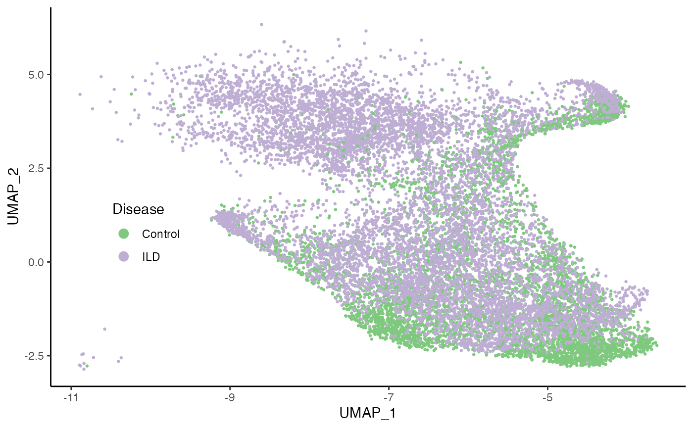

ggplot(df, aes(x = UMAP_1, y = UMAP_2, col = celltype)) +
  geom_point(size = .5) +
  scale_color_brewer(palette = "Dark2") +
  labs(col = "Cell Type") +
  theme(legend.position = c(.2, .4),
        legend.background = element_blank()) +
  guides(col = guide_legend(override.aes = list(size = 3)))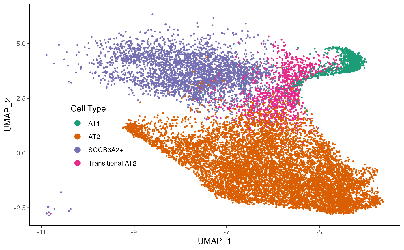

Imbalance score

scores <- condiments::imbalance_score(
  Object = df %>% select(UMAP_1, UMAP_2) %>% as.matrix(), 
  conditions = df$Status, k = 20, smooth = 30)
df$scores <- scores$scaled_scores
ggplot(df, aes(x = UMAP_1, y = UMAP_2, col = scores)) +
  geom_point(size = .7) +
  scale_color_viridis_c(option = "C", breaks = c(0, 2, 4, 6)) +
  labs(col = "Scores") +
  theme(legend.position = c(.15, .4),
        legend.background = element_blank())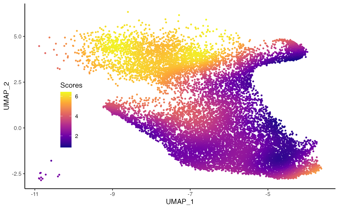

Differential Topology

To estimate the trajectory, we use slingshot (Street et al. 2018).

Fit slingshot

fibrosis <- slingshot(fibrosis, reducedDim = 'UMAP',
                 clusterLabels = colData(fibrosis)$celltype,
                 start.clus = 'AT1', approx_points = 100)

Topology Test

set.seed(821)
topologyTest(SlingshotDataSet(fibrosis), fibrosis$Status)

## Generating permuted trajectories

## Running KS-mean test

##    method thresh  statistic      p.value
## 1 KS_mean   0.01 0.04183036 2.964406e-12

fibrosis_SCGB3A2 <- slingshot(fibrosis[, fibrosis$celltype != "SCGB3A2+"],
                         reducedDim = 'UMAP',
            clusterLabels = colData(fibrosis[, fibrosis$celltype != "SCGB3A2+"])$celltype,
                 start.clus = 'AT1', approx_points = 100)
set.seed(821)
topologyTest(SlingshotDataSet(fibrosis_SCGB3A2), fibrosis_SCGB3A2$Status)

## Generating permuted trajectories
## Running KS-mean test

##    method thresh   statistic p.value
## 1 KS_mean   0.01 0.002720157       1

rm(fibrosis_SCGB3A2)

Separate trajectories

sdss <- slingshot_conditions(SlingshotDataSet(fibrosis), fibrosis$Status)
curves <- bind_rows(lapply(sdss, slingCurves, as.df = TRUE),
                    .id = "Status")

p4a <- ggplot(df, aes(x = UMAP_1, y = UMAP_2, col = Status)) +
  geom_point(size = .7, alpha = .2) +
  scale_color_brewer(palette = "Accent") +
  labs(col = "Disaes") +
  geom_path(data = curves %>% arrange(Status, Lineage, Order),
            aes(group = interaction(Lineage, Status)), size = 1.5) +
  annotate("text", x = -10, y = 6, label = "Lineage1", size = 5) +
  annotate("text", x = -7, y = -2.7, label = "Lineage2", size = 5) +
  theme(legend.position = c(.15, .35),
        legend.background = element_blank()) +
  NULL
p4a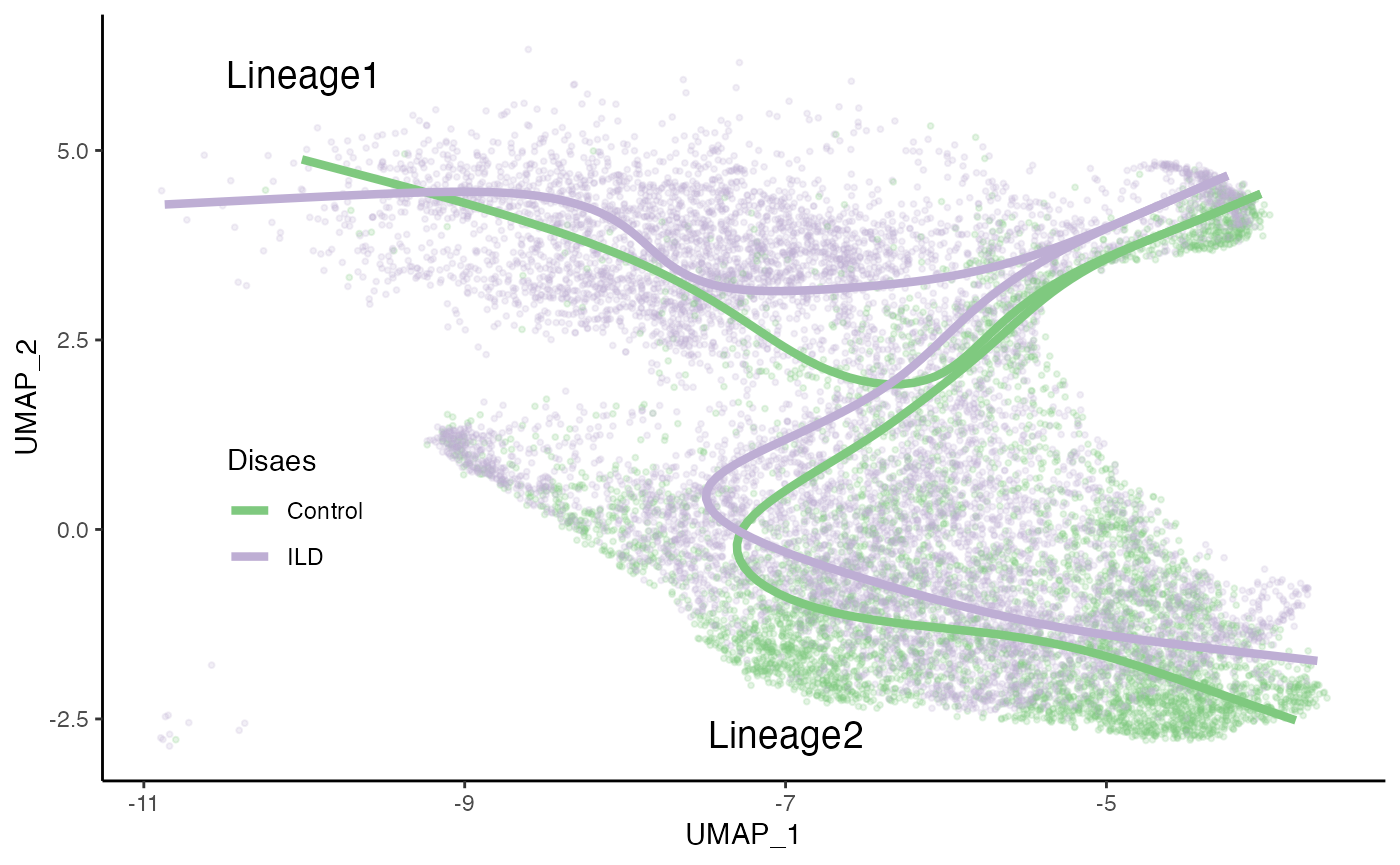

Common trajectory

df <- bind_cols(
  as.data.frame(reducedDim(fibrosis, "UMAP")),
  slingPseudotime(fibrosis) %>% as.data.frame() %>%
    dplyr::rename_with(paste0, "_pst", .cols = everything()),
  slingCurveWeights(fibrosis) %>% as.data.frame(),
  ) %>%
  mutate(Lineage1_pst = if_else(is.na(Lineage1_pst), 0, Lineage1_pst),
         Lineage2_pst = if_else(is.na(Lineage2_pst), 0, Lineage2_pst),
         pst = if_else(Lineage1 > Lineage2, Lineage1_pst, Lineage2_pst),
         pst = max(pst) - pst)
curves <- slingCurves(fibrosis, as.df = TRUE)
ggplot(df, aes(x = UMAP_1, y = UMAP_2)) +
  geom_point(size = .7, aes(col = pst)) +
  scale_color_viridis_c() +
  labs(col = "Pseudotime") +
  geom_path(data = curves %>% arrange(Order),
            aes(group = Lineage), col = "black", size = 1.5) +
  annotate("text", x = -10, y = 6, label = "Lineage1", size = 5) +
  annotate("text", x = -7, y = -2.7, label = "Lineage2", size = 5) +
  theme(legend.position = c(.15, .35),
        legend.background = element_blank())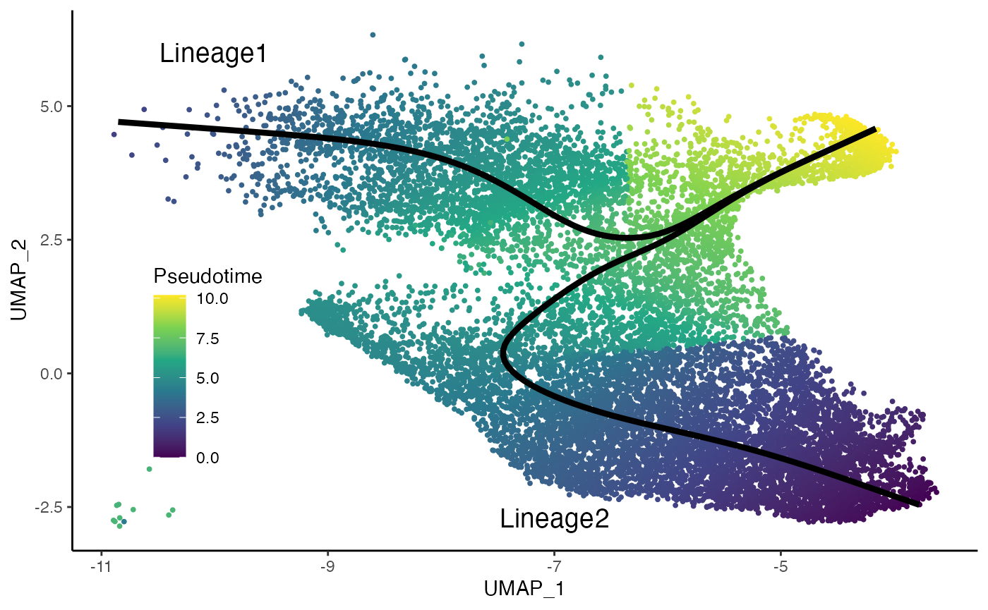

Differential Progression

Test

progressionTest(fibrosis, conditions = fibrosis$Status, lineages = TRUE)

##   lineage  statistic     p.value
## 1     All 10.6182770 1.22521e-26
## 2       1  0.6388885 2.20000e-16
## 3       2  0.1998837 2.20000e-16

Plot

df <-  slingPseudotime(fibrosis) %>% as.data.frame() 
df$Status <- fibrosis$Status
df <- df %>% 
  pivot_longer(-Status, names_to = "Lineage",
               values_to = "pst") %>%
  filter(!is.na(pst))
ggplot(df, aes(x = pst)) +
  geom_density(alpha = .8, aes(fill = Status), col = "transparent") +
  geom_density(aes(col = Status), fill = "transparent", size = 1.5) +
  labs(x = "Pseudotime", fill = "Status") +
  facet_wrap(~Lineage, scales = "free_x") +
  guides(col = "none", fill = guide_legend(
    override.aes = list(size = 1.5, col = c("#7FC97F", "#BEAED4"))
  )) +
  scale_fill_brewer(palette = "Accent") +
  scale_color_brewer(palette = "Accent") +
  theme(legend.position = c(.8, .8), legend.direction = "horizontal")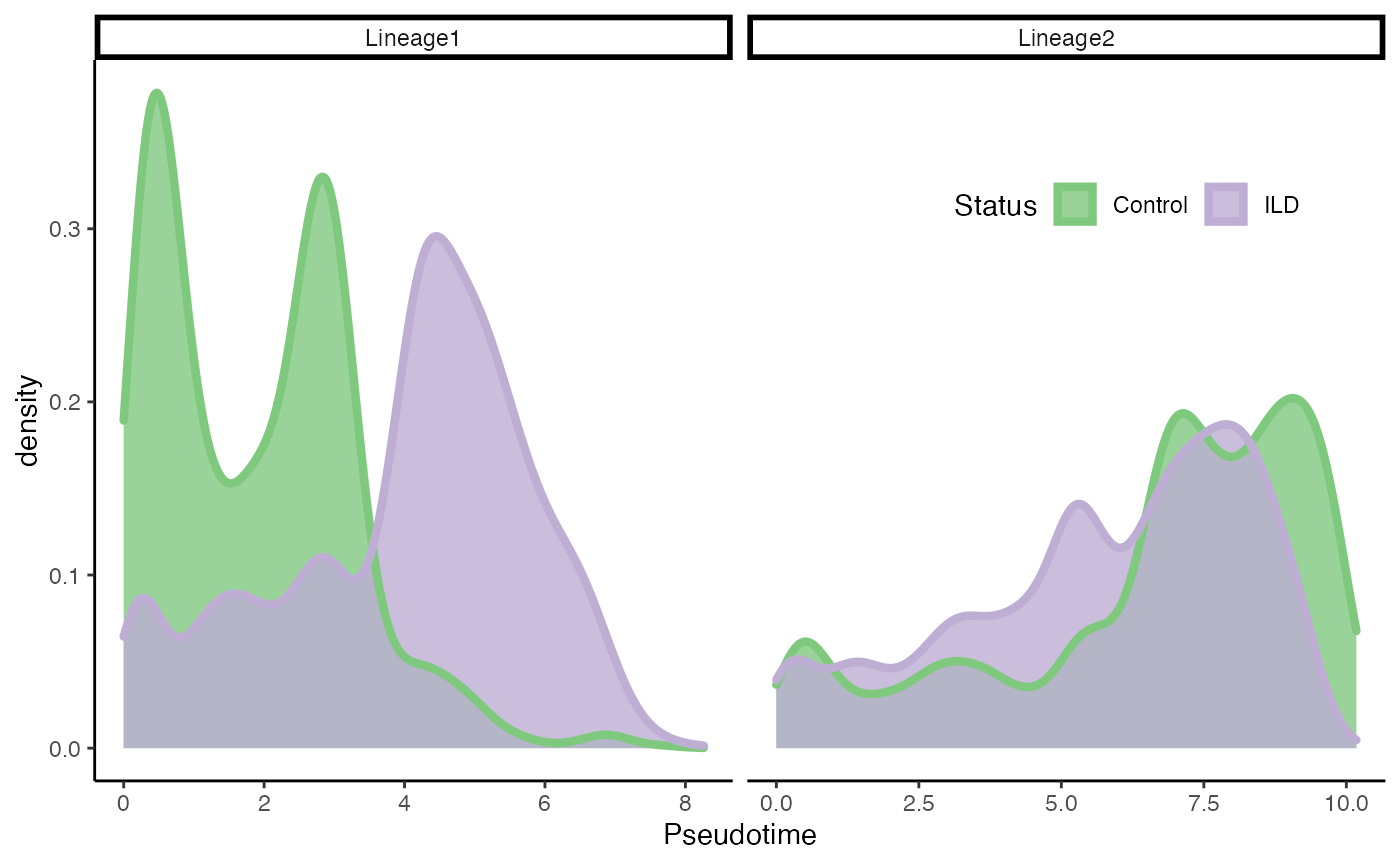

Differential fate selection

Test

fateSelectionTest(fibrosis, conditions = fibrosis$Status)

## note: only 1 unique complexity parameters in default grid. Truncating the grid to 1 .

## Loading required package: lattice

## note: only 1 unique complexity parameters in default grid. Truncating the grid to 1 .

## Registered S3 method overwritten by 'cli':
##   method     from         
##   print.boxx spatstat.geom

## # A tibble: 1 × 3
##   pair  statistic  p.value
##   <chr>     <dbl>    <dbl>
## 1 1vs2      0.647 7.95e-64

Plot

df <- slingCurveWeights(SlingshotDataSet(fibrosis), as.probs = TRUE) %>% as.data.frame()
df$Status <- fibrosis$Status
df <- df %>%
  pivot_longer(-Status, names_to = "Lineage", values_to = "ws")
ggplot(df, aes(x = ws)) +
  geom_density(alpha = .8, aes(fill = Status), col = "transparent") +
  geom_density(aes(col = Status), fill = "transparent", size = 1.5) +
  labs(x = "Weights", fill = "Status") +
  facet_wrap(~Lineage, scales = "free_x") +
  guides(fill = "none", col = "none") +
  scale_fill_brewer(palette = "Accent") +
  scale_color_brewer(palette = "Accent")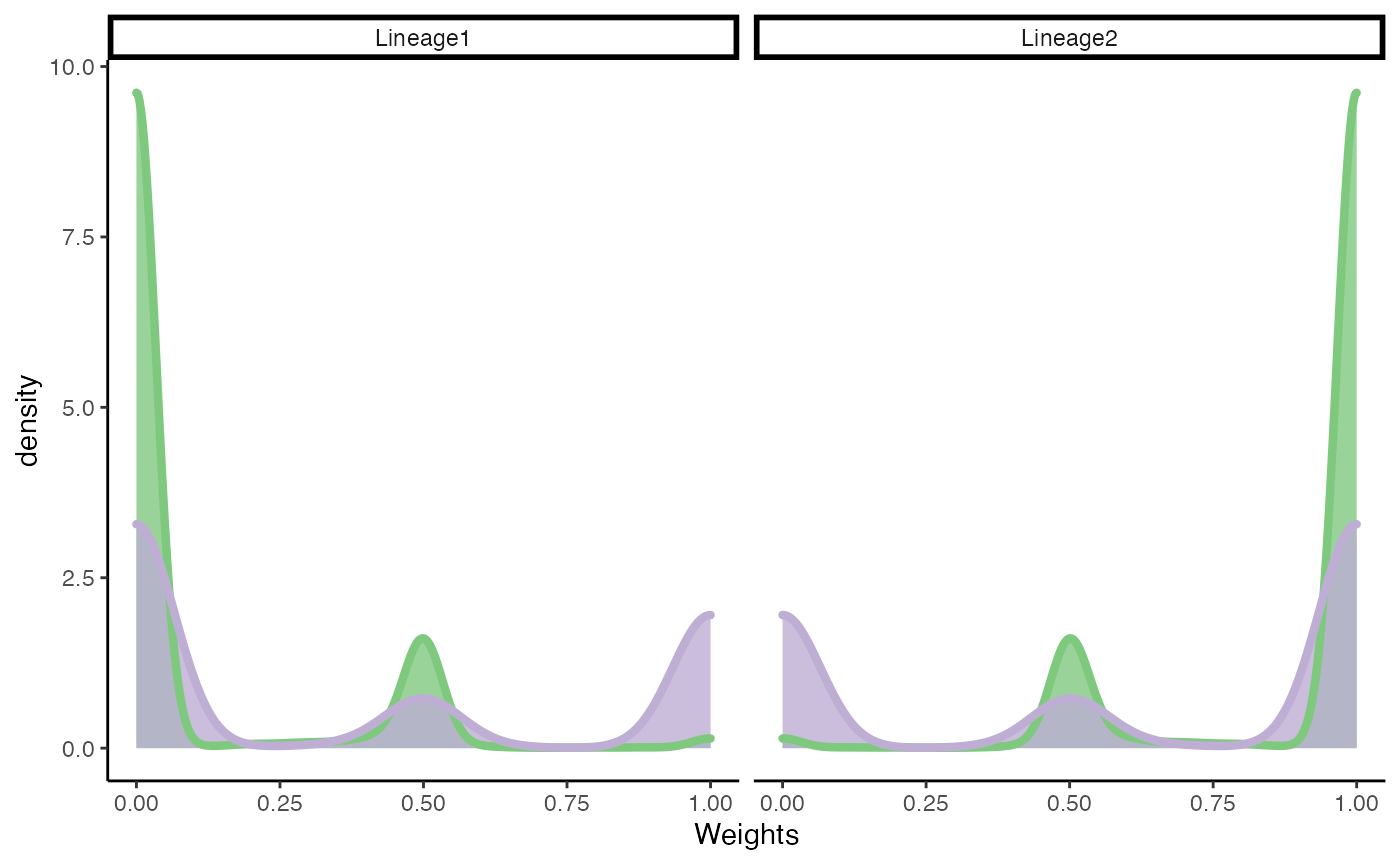

Differential expression

We use tradeSeq (Van den Berge et al. 2020).

Select number of knots

library(tradeSeq)
set.seed(3)
BPPARAM <- BiocParallel::bpparam()
BPPARAM$workers <- 3
icMat <- evaluateK(counts = fibrosis, sds = SlingshotDataSet(fibrosis), 
                   conditions = factor(fibrosis$Status),
                   nGenes = 300, parallel = TRUE, BPPARAM = BPPARAM, k = 3:7)

Fit GAM

Next, we fit the NB-GAMs using 6 knots, based on the pseudotime and cell-level weights estimated by Slingshot. We use the conditions argument to fit separate smoothers for each condition.

library(tradeSeq)
set.seed(3)
fibrosis <- fitGAM(counts = fibrosis, conditions = factor(fibrosis$Status), nknots = 6)

Differential expression between conditions

condRes <- conditionTest(fibrosis, l2fc = log2(2), lineages = TRUE)
condRes$padj <- p.adjust(condRes$pvalue_lineage1, "fdr")
mean(condRes$padj <= 0.05, na.rm = TRUE)

## [1] 0.0002972946

sum(condRes$padj <= 0.05, na.rm = TRUE)

## [1] 3

conditionGenes <- rownames(condRes)[condRes$padj <= 0.05]
conditionGenes <- conditionGenes[!is.na(conditionGenes)]

Differential expression between lineages

patRes <- patternTest(fibrosis, l2fc = log2(2))
patRes$padj <- p.adjust(patRes$pvalue, "fdr")
mean(patRes$padj <= 0.05, na.rm = TRUE)

## [1] 0.1574202

sum(patRes$padj <= 0.05, na.rm = TRUE)

## [1] 1589

patternGenes <- rownames(patRes)[patRes$padj <= 0.05]
patternGenes <- patternGenes[!is.na(patternGenes)]

Visualize select genes from the og paper

library(RColorBrewer)
scales <- c("#FCAE91", "#DE2D26", "#BDD7E7", "#3182BD")

# plot genes
oo <- order(patRes$waldStat, decreasing = TRUE)
genes <- c("SCGB3A2", "SFTPC", "ABCA3", "AGER")

# most significant gene
ps <- lapply(genes, function(gene){
  plotSmoothers(fibrosis, assays(fibrosis)$counts, gene = gene, curvesCol = scales,
                border = FALSE, sample = .2) +
    scale_x_reverse(breaks = 0:4/.4, labels = 4:0/.4) +
    labs(title = gene, col = "Lineage and Condition") +
    scale_color_manual(values = scales) +
    theme(plot.title = element_text(hjust = .5),
          rect = element_blank())
  }
)

## Scale for 'colour' is already present. Adding another scale for 'colour',
## which will replace the existing scale.
## Scale for 'colour' is already present. Adding another scale for 'colour',
## which will replace the existing scale.
## Scale for 'colour' is already present. Adding another scale for 'colour',
## which will replace the existing scale.
## Scale for 'colour' is already present. Adding another scale for 'colour',
## which will replace the existing scale.

legend_gene <- get_legend(
  ps[[1]] + theme(legend.position = "bottom") +
    guides(col = guide_legend(title.position = "top"))
)
ps <- lapply(ps, function(p) {p + guides(col = "none")})
p6 <- plot_grid(
  plot_grid(plotlist = ps, ncol = 2, scale = .95,
            labels = c('a)', 'b)', 'c)', 'd)')),
  plot_grid(NULL, legend_gene, NULL, rel_widths = c(1, 1, 1), ncol = 3), 
  nrow = 2, rel_heights = c(4, .5)
)

Heatmaps of genes DE between lineages

Below we show heatmaps of the genes DE between lineages The DE genes in the heatmaps are ordered according to a hierarchical clustering on the first lineage.

### based on mean smoother
yhatSmooth <- predictSmooth(fibrosis, gene = patternGenes, nPoints = 50, tidy = TRUE) %>%
  mutate(yhat = log1p(yhat)) %>%
  group_by(gene) %>%
  mutate(yhat = scales::rescale(yhat)) %>%
  filter(condition == "ILD") %>%
  select(-condition) %>%
  ungroup()
heatSmooth_Lineage1 <- pheatmap(
  yhatSmooth %>%
    filter(lineage == 1) %>%
    select(-lineage) %>%
    arrange(-time) %>%
    pivot_wider(names_from = time, values_from = yhat) %>%
    select(-gene),
  cluster_cols = FALSE, show_rownames = FALSE, show_colnames = FALSE,
  main = "Lineage 1", legend = FALSE, silent = TRUE
)

heatSmooth_Lineage2 <- pheatmap(
  (yhatSmooth %>%
    filter(lineage == 2) %>%
    select(-lineage) %>%
    arrange(-time) %>%
    pivot_wider(names_from = time, values_from = yhat) %>%
    select(-gene))[heatSmooth_Lineage1$tree_row$order, ],
  cluster_cols = FALSE, cluster_rows = FALSE,
  show_rownames = FALSE, show_colnames = FALSE, main = "Lineage 2",
  legend = FALSE, silent = TRUE 
)

p7 <- plot_grid(heatSmooth_Lineage1[[4]], heatSmooth_Lineage2[[4]], ncol = 2)
p7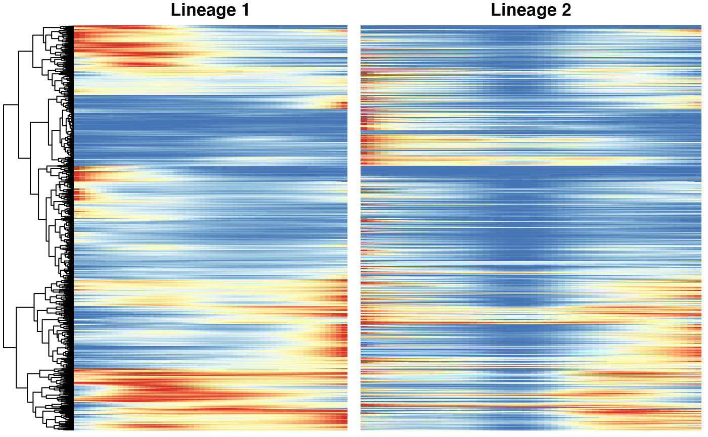

Session info

sessionInfo()

## R version 4.1.0 (2021-05-18)
## Platform: x86_64-apple-darwin17.0 (64-bit)
## Running under: macOS Big Sur 10.16
## 
## Matrix products: default
## BLAS:   /Library/Frameworks/R.framework/Versions/4.1/Resources/lib/libRblas.dylib
## LAPACK: /Library/Frameworks/R.framework/Versions/4.1/Resources/lib/libRlapack.dylib
## 
## locale:
## [1] en_US.UTF-8/en_US.UTF-8/en_US.UTF-8/C/en_US.UTF-8/en_US.UTF-8
## 
## attached base packages:
## [1] parallel  stats4    stats     graphics  grDevices utils     datasets 
## [8] methods   base     
## 
## other attached packages:
##  [1] RColorBrewer_1.1-2          caret_6.0-88               
##  [3] lattice_0.20-44             scales_1.1.1               
##  [5] msigdbr_7.4.1               fgsea_1.18.0               
##  [7] pheatmap_1.0.12             tradeSeq_1.7.04            
##  [9] readr_2.0.0                 condiments_1.1.04          
## [11] cowplot_1.1.1               slingshot_2.1.1            
## [13] TrajectoryUtils_1.0.0       princurve_2.1.6            
## [15] scater_1.20.1               ggplot2_3.3.5              
## [17] scuttle_1.2.0               SingleCellExperiment_1.14.1
## [19] SummarizedExperiment_1.22.0 Biobase_2.52.0             
## [21] GenomicRanges_1.44.0        GenomeInfoDb_1.28.2        
## [23] IRanges_2.26.0              S4Vectors_0.30.0           
## [25] BiocGenerics_0.38.0         MatrixGenerics_1.4.3       
## [27] matrixStats_0.60.1          SeuratObject_4.0.2         
## [29] Seurat_4.0.3                dplyr_1.0.7                
## [31] tidyr_1.1.3                 here_1.0.1                 
## [33] knitr_1.33                 
## 
## loaded via a namespace (and not attached):
##   [1] utf8_1.2.2                reticulate_1.20          
##   [3] tidyselect_1.1.1          htmlwidgets_1.5.3        
##   [5] grid_4.1.0                BiocParallel_1.26.2      
##   [7] Rtsne_0.15                pROC_1.17.0.1            
##   [9] munsell_0.5.0             ScaledMatrix_1.0.0       
##  [11] codetools_0.2-18          ragg_1.1.3               
##  [13] ica_1.0-2                 future_1.21.0            
##  [15] miniUI_0.1.1.1            withr_2.4.2              
##  [17] colorspace_2.0-2          highr_0.9                
##  [19] rstudioapi_0.13           ROCR_1.0-11              
##  [21] tensor_1.5                listenv_0.8.0            
##  [23] labeling_0.4.2            GenomeInfoDbData_1.2.6   
##  [25] polyclip_1.10-0           farver_2.1.0             
##  [27] rprojroot_2.0.2           parallelly_1.27.0        
##  [29] vctrs_0.3.8               generics_0.1.0           
##  [31] ipred_0.9-11              xfun_0.24                
##  [33] Ecume_0.9.1               randomForest_4.6-14      
##  [35] R6_2.5.1                  ggbeeswarm_0.6.0         
##  [37] rsvd_1.0.5                locfit_1.5-9.4           
##  [39] bitops_1.0-7              spatstat.utils_2.2-0     
##  [41] cachem_1.0.5              DelayedArray_0.18.0      
##  [43] assertthat_0.2.1          promises_1.2.0.1         
##  [45] nnet_7.3-16               beeswarm_0.4.0           
##  [47] gtable_0.3.0              beachmat_2.8.0           
##  [49] globals_0.14.0            goftest_1.2-2            
##  [51] timeDate_3043.102         rlang_0.4.11             
##  [53] systemfonts_1.0.2         splines_4.1.0            
##  [55] lazyeval_0.2.2            ModelMetrics_1.2.2.2     
##  [57] spatstat.geom_2.2-2       yaml_2.2.1               
##  [59] reshape2_1.4.4            abind_1.4-5              
##  [61] httpuv_1.6.1              tools_4.1.0              
##  [63] lava_1.6.9                ellipsis_0.3.2           
##  [65] spatstat.core_2.3-0       jquerylib_0.1.4          
##  [67] proxy_0.4-26              ggridges_0.5.3           
##  [69] Rcpp_1.0.7                plyr_1.8.6               
##  [71] sparseMatrixStats_1.4.0   zlibbioc_1.38.0          
##  [73] purrr_0.3.4               RCurl_1.98-1.4           
##  [75] rpart_4.1-15              deldir_0.2-10            
##  [77] pbapply_1.4-3             viridis_0.6.1            
##  [79] zoo_1.8-9                 ggrepel_0.9.1            
##  [81] cluster_2.1.2             fs_1.5.0                 
##  [83] magrittr_2.0.1            data.table_1.14.0        
##  [85] scattermore_0.7           lmtest_0.9-38            
##  [87] RANN_2.6.1                fitdistrplus_1.1-5       
##  [89] hms_1.1.0                 patchwork_1.1.1          
##  [91] mime_0.11                 evaluate_0.14            
##  [93] xtable_1.8-4              gridExtra_2.3            
##  [95] transport_0.12-2          compiler_4.1.0           
##  [97] tibble_3.1.4              KernSmooth_2.23-20       
##  [99] crayon_1.4.1              htmltools_0.5.1.1        
## [101] tzdb_0.1.2                mgcv_1.8-36              
## [103] later_1.2.0               lubridate_1.7.10         
## [105] DBI_1.1.1                 MASS_7.3-54              
## [107] babelgene_21.4            Matrix_1.3-4             
## [109] cli_3.0.1                 gower_0.2.2              
## [111] igraph_1.2.6              pkgconfig_2.0.3          
## [113] pkgdown_1.6.1             plotly_4.9.4.1           
## [115] spatstat.sparse_2.0-0     recipes_0.1.16           
## [117] foreach_1.5.1             vipor_0.4.5              
## [119] bslib_0.2.5.1             XVector_0.32.0           
## [121] prodlim_2019.11.13        stringr_1.4.0            
## [123] digest_0.6.27             sctransform_0.3.2        
## [125] RcppAnnoy_0.0.18          spatstat.data_2.1-0      
## [127] fastmatch_1.1-0           rmarkdown_2.9            
## [129] leiden_0.3.8              edgeR_3.34.0             
## [131] uwot_0.1.10               DelayedMatrixStats_1.14.0
## [133] kernlab_0.9-29            shiny_1.6.0              
## [135] lifecycle_1.0.0           nlme_3.1-152             
## [137] jsonlite_1.7.2            BiocNeighbors_1.10.0     
## [139] limma_3.48.3              desc_1.3.0               
## [141] viridisLite_0.4.0         fansi_0.5.0              
## [143] spatstat.linnet_2.3-0     pillar_1.6.2             
## [145] fastmap_1.1.0             httr_1.4.2               
## [147] survival_3.2-11           glue_1.4.2               
## [149] spatstat_2.2-0            png_0.1-7                
## [151] iterators_1.0.13          class_7.3-19             
## [153] stringi_1.7.3             sass_0.4.0               
## [155] textshaping_0.3.5         BiocSingular_1.8.1       
## [157] memoise_2.0.0             e1071_1.7-7              
## [159] irlba_2.3.3               future.apply_1.7.0

References

Street, Kelly, Davide Risso, Russell B. Fletcher, Diya Das, John Ngai, Nir Yosef, Elizabeth Purdom, and Sandrine Dudoit. 2018. “Slingshot: cell lineage and pseudotime inference for single-cell transcriptomics.” BMC Genomics 19 (1): 477. https://doi.org/10.1186/s12864-018-4772-0.

Van den Berge, Koen, Hector Roux de Bézieux, Kelly Street, Wouter Saelens, Robrecht Cannoodt, Yvan Saeys, Sandrine Dudoit, and Lieven Clement. 2020. “Trajectory-based differential expression analysis for single-cell sequencing data.” Nature Communications 11 (1): 1201. https://doi.org/10.1038/s41467-020-14766-3.

Analysis of the fibrosis datataset

Hector Roux de Bézieux

Load data

EDA

Imbalance score

Differential Topology

Fit slingshot

Topology Test

Separate trajectories

Common trajectory

Differential Progression

Test

Plot

Differential fate selection

Test

Plot

Differential expression

Select number of knots

Fit GAM

Differential expression between conditions

Differential expression between lineages

Visualize select genes from the og paper

Heatmaps of genes DE between lineages

Session info

References