Second example: KRAS dataset
Hector Roux de Bézieux
KRAS.RmdOverview
The dataset we will be working with concerns a single-cell RNA-sequencing dataset consisting of three cancer models under a KRAS(G12C) inhibition (Xue et al. 2020). Those types of molecules are currently in early-phase clinical trials and a large group of lung adenocarcinoma seem to be able to at least partially evade those treatments. The authors of the original study therefore look at the impact of KRAS(G12C) inhibitors on three models of tumors and show that cells evolve along three lineages.
While the authors used the three models to validate their results, we can also look for differences between the three types. We therefore have a three-lineages trajectory, with three conditions (i.e. the three tumor models).
We will use this dataset as an example of how to perform the first two steps of the condiments workflow under this setting. + We first check if we can fit a single trajectory, which we call differential topology. + We then look for large-scale changes, indicative of differential progression and differential differentiation.
Load data
libs <- c("here", "dplyr", "tradeSeq", "SingleCellExperiment", "slingshot",
           "condiments", "scater", "RColorBrewer", "pheatmap", "cowplot",
          "tidyr", "ggplot2")
suppressMessages(
  suppressWarnings(sapply(libs, require, character.only = TRUE))
)
## here dplyr tradeSeq
## FALSE TRUE TRUE
## SingleCellExperiment slingshot condiments
## TRUE TRUE TRUE
## scater RColorBrewer pheatmap
## FALSE TRUE TRUE
## cowplot tidyr ggplot2
## TRUE TRUE TRUE
rm(libs)
theme_set(theme_classic())
kras <- bioc2021trajectories::import_KRAS()
kras <- kras[1:100, ]
We rely on normalization conducted in the original paper, and will use the reduced dimension coordinates that are available. We provide a function to access both the raw counts, the reduced dimension coordinates and other cell-level info. Since we will not be performing differential expression, we do not need to retain the genes and we only keep a lightweight version of the object.
data("kras", package = "bioc2021trajectories")
kras## class: SingleCellExperiment
## dim: 100 10177
## metadata(0):
## assays(1): counts
## rownames(100): NOC2L HES4 ... MECR PUM1
## rowData names(20): ensembl gene_short_name ... br.qval br.qval.72
## colnames(10177): H358_A_AAACATACATAAGG H358_A_AAACATACATACCG ...
## SW1573_D_TTTAGAGATCAGAC SW1573_D_TTTCGAACTTCTGT
## colData names(98): nGene nUMI ... slingshot cells
## reducedDimNames(1): TSNE
## mainExpName: NULL
## altExpNames(0):EDA
We can visualize all the single cells in a shared reduced dimensional space, according to the tumor model or the clusters from the original publication.
cols <- c(brewer.pal(5, "Blues")[2:5],
          brewer.pal(3, "Greens")[2:3],
          brewer.pal(3, "Reds")[2:3],
          brewer.pal(3, "Oranges")[2], "Grey")
names(cols) <- c(3, 5, 4, 1, 8, 2, 9, 10, 6, 7)
df <- colData(kras)[, -97] %>% as.data.frame() %>%
  sample_frac(1)
ggplot(df, aes(x = tSNE1, y = tSNE2, col = Batch)) +
  geom_point(size = .7) +
  scale_color_brewer(palette = "Accent") +
  labs(col = "Type")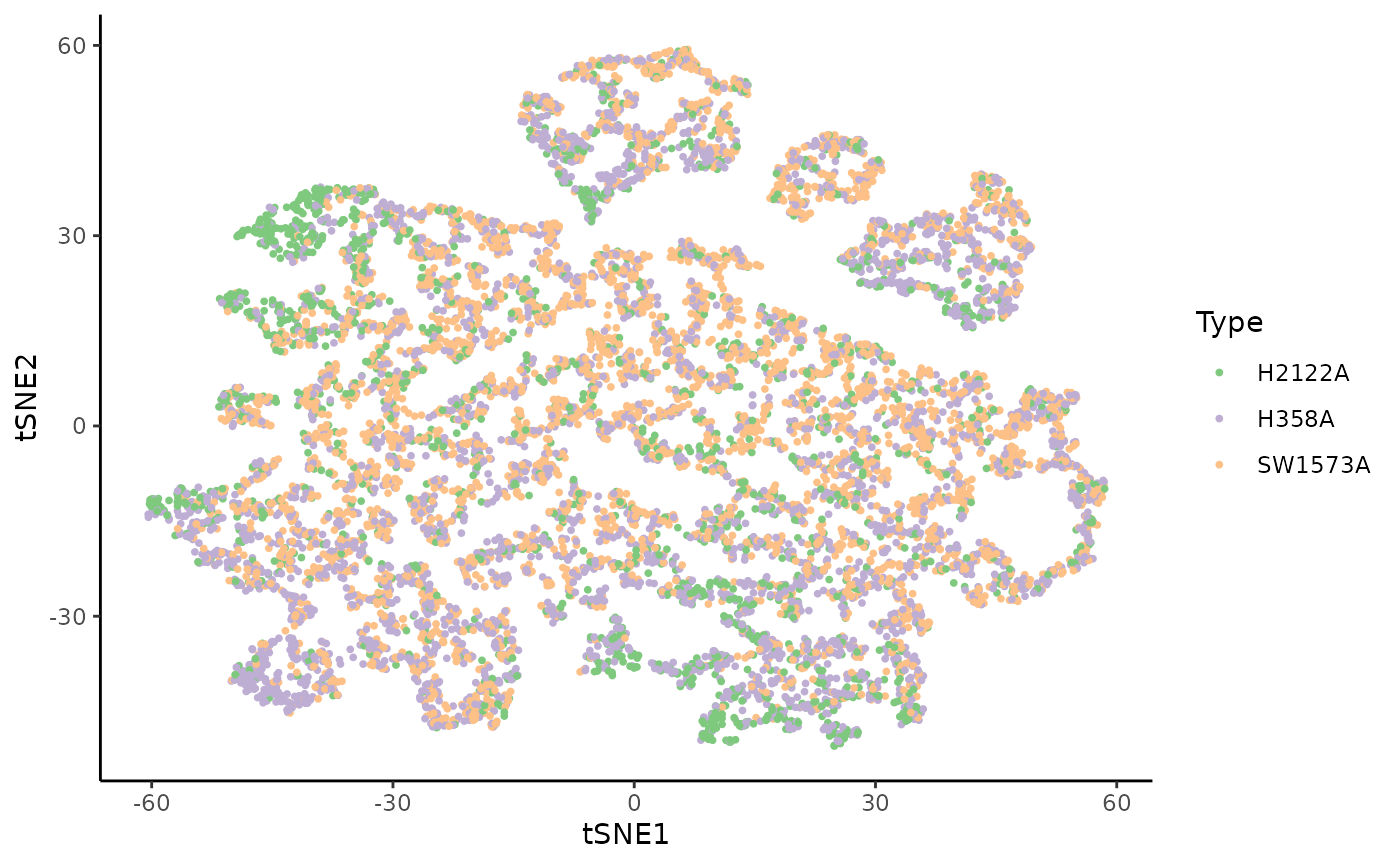
ggplot(df, aes(x = tSNE1, y = tSNE2, fill = Cluster)) +
  geom_point(size = 1, alpha = .65, col = "grey70", shape = 21) +
  scale_fill_manual(values = cols) +
  labs(fill = "Cell Clusters")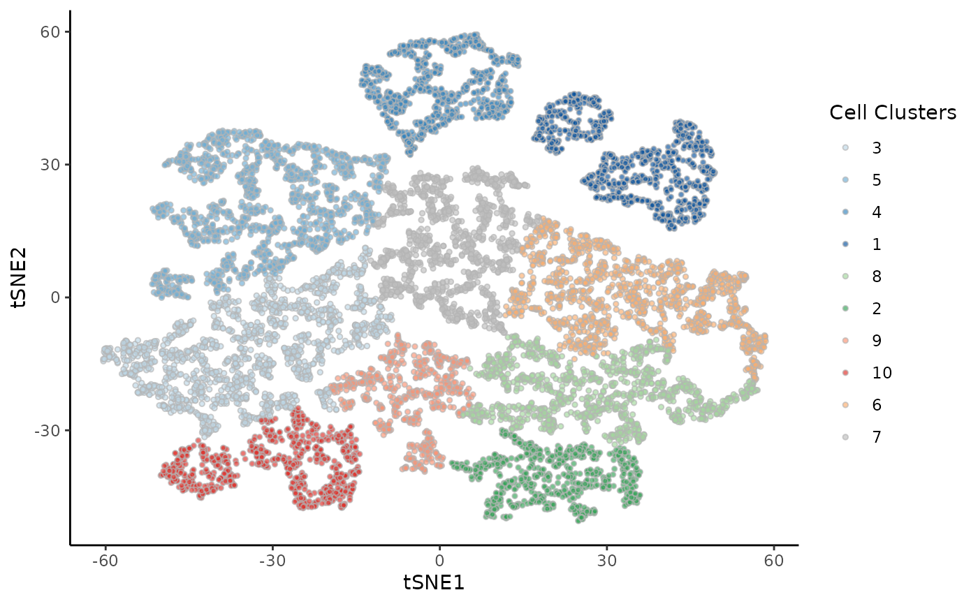
Differential Topology
The first question we ask is whether we can fit a common trajectory. If the differences between the models are limited, then a common trajectory is possible. If there are large changes, then it is better to fit one trajectory per tumor model. In the latter case, depending on the scale of those changes, it may still be possible to reconcile the trajectories manually.
To assess this, we first use a visual tool called the imbalance_score.
Imbalance score
kras <- imbalance_score(Object = kras, conditions = "Batch", dimred = "TSNE")
df$scores <- kras[, df$cells]$scores$scaled_scores
ggplot(df, aes(x = tSNE1, y = tSNE2, col = scores)) +
  geom_point(size = .7) +
  scale_color_viridis_c(option = "C") +
  labs(col = "Score")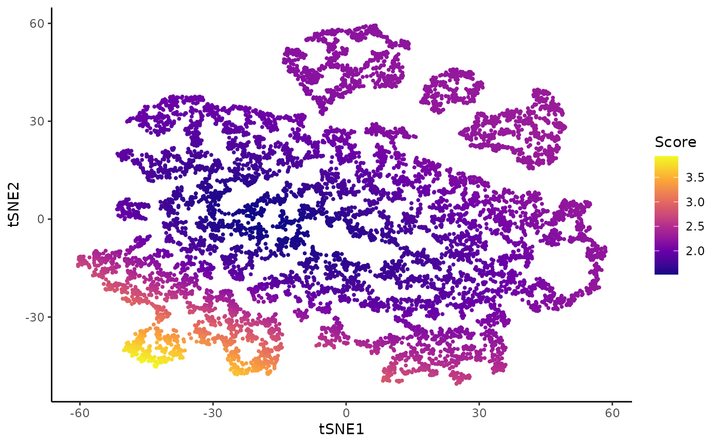
There are some clear regions of imbalance (especially in cluster 10), although overall the three conditions are well mixed.
To assess whether a common trajectory can be fitted in a more quantitative manner, we will rely on the topologyTest. To do this, we fit a common trajectory (under the null) which will serve as a guide for condition-level trajectories. To estimate the trajectory, we use slingshot (Street et al. 2018).
Fit slingshot and visualize the trajectory skeleton.
kras <- slingshot(kras, reducedDim = "TSNE", clusterLabels = kras$Cluster,
                 start.clus = 7, extend = "n", reweight = FALSE, reassign = FALSE)
mst <- slingMST(kras, as.df = TRUE)
ggplot(df, aes(x = tSNE1, y = tSNE2)) +
  geom_point(size = 1, alpha = .65, col = "grey70", shape = 21,
             aes(fill = Cluster)) +
  scale_fill_manual(values = cols) +
  labs(fill = "Cell Clusters") +
  geom_point(size = 3, data = mst) +
  geom_path(size = 1.5, data = mst, aes(group = Lineage))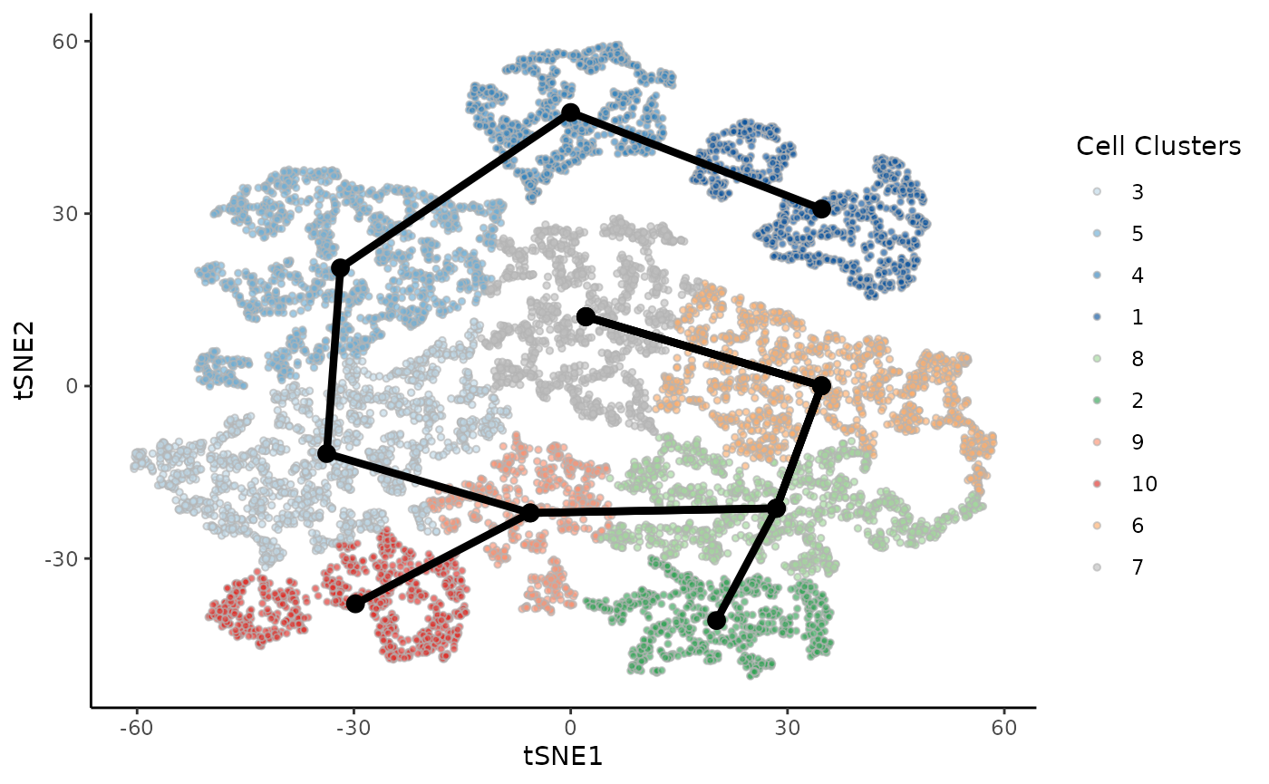
The skeleton of the trajectory is this tree structure, that tracks changes, consistently with the original publication. The topologyTest utilizes this tree structure when fitting curves to the cells of each condition, as well as to random sets of the data, and compares whether the two distributions are similar.
Topology Test
set.seed(23)
topologyTest(kras, conditions = "Batch", rep = 50)
## Generating permuted trajectories## Running Classifier test## Loading required package: lattice## method thresh statistic p.value
## 1 Classifier 0.01 0.9181035 0Here, we clearly reject the topologyTest: we should fit a separate trajectory per condition.
Individual curves
Fit
We therefore fit one trajectory per tumor model, or batch, using the slingshot_conditions function.
sdss <- slingshot_conditions(kras, kras$Batch, approx_points = FALSE,
                             extend = "n", reweight = FALSE, reassign = FALSE)
Plot skeletons
We can plot the skeleton of each trajectory. They are clearly very similar and we can visually map the trajectories: the lineages map well onto one another.
msts <- lapply(sdss, slingMST, as.df = TRUE) %>%
  bind_rows(.id = "Batch") %>%
  arrange(Batch)

ggplot(df, aes(x = tSNE1, y = tSNE2, col = Batch)) +
  geom_point(size = .7, alpha = .1) +
  scale_color_brewer(palette = "Accent") +
  geom_point(data = msts, size = 3) +
  geom_path(data = msts, aes(group = interaction(Lineage, Batch)),
            size = 2)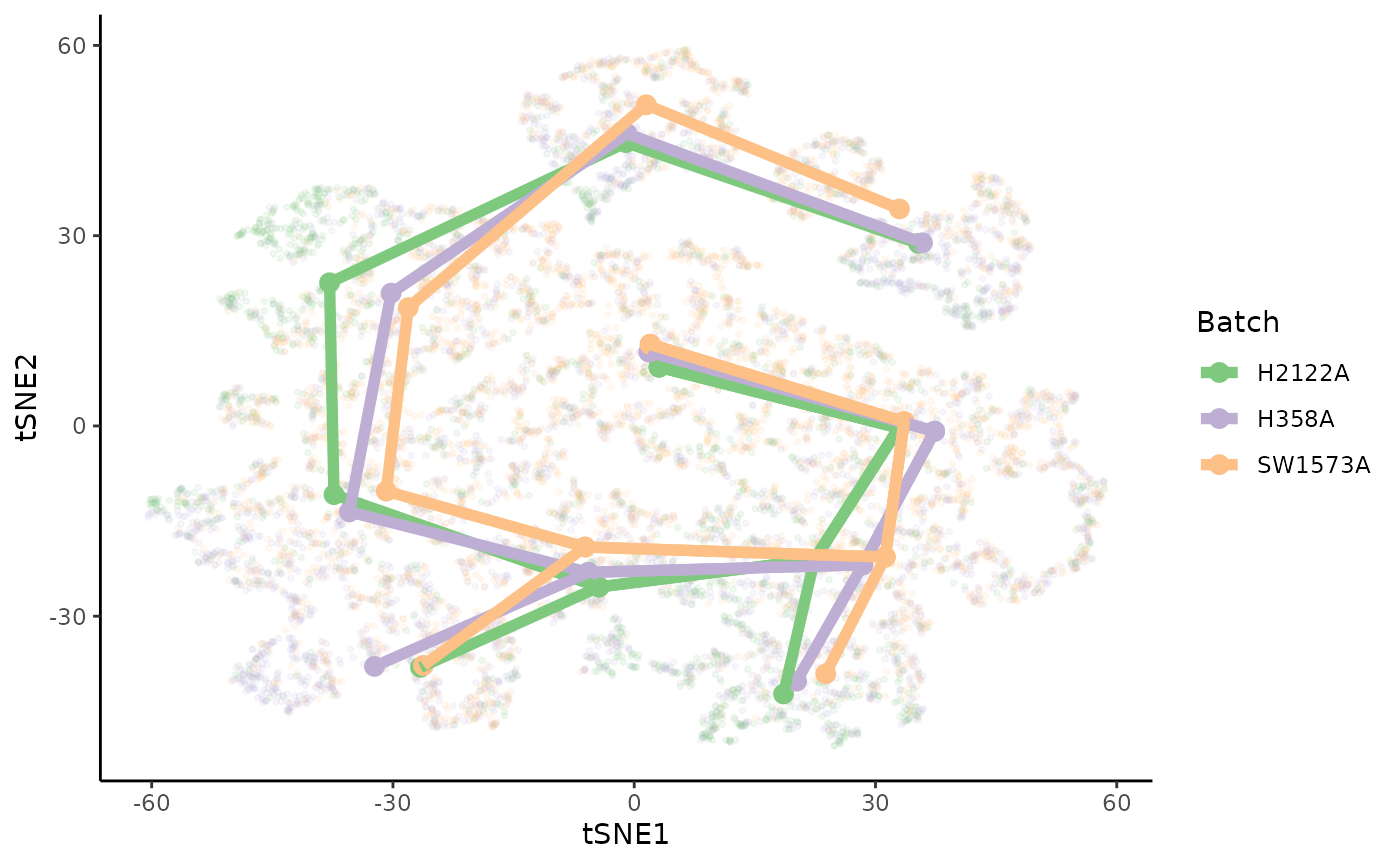
Plot curves
Similarly with the curves, we see that the three lineages of each trajectory map to one another across conditions.
lineages <- lapply(sdss, slingCurves, as.df = TRUE) %>%
  bind_rows(.id = "Batch") %>%
  arrange(Order)
position <- data.frame(
  "tSNE1" = c(40, -30, 45),
  "tSNE2" = c(50, -50, -50),
  "Batch" = "H2122A",
  "text" = paste0("Lineage ", 1:3)
)

ggplot(df, aes(x = tSNE1, y = tSNE2, col = Batch)) +
  geom_point(size = .7, alpha = .2) +
  scale_color_brewer(palette = "Accent") +
  geom_path(data = lineages, size = 1.5, aes(group = interaction(Lineage, Batch))) +
  geom_text(data = position, col = "black", aes(label = text), size = 5)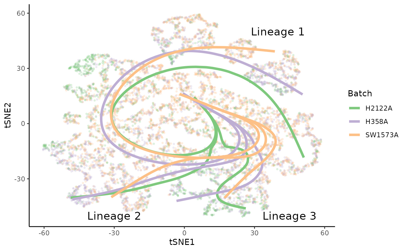
Manual mapping
Although we have fitted a different trajectory per condition, we can therefore proceed to step 2 and look at differential progression and differentiation, by manually mapping the trajectories.
##      [,1] [,2] [,3]
## [1,]    1    1    1
## [2,]    2    2    2
## [3,]    3    3    3
sds <- merge_sds(sdss[[1]], sdss[[2]], sdss[[3]],
                 condition_id = names(sdss), mapping = mapping)
Differential Progression
Similarly to the TGFB dataset, we can look at large-scale differences between conditions. Specifically, we want to see if the pseudotime distributions are similar across conditions.
Plot
df <- full_join(
  df %>%
    select(cells, tSNE1, tSNE2, Cluster, Batch),
  slingPseudotime(sds) %>%
    as.data.frame() %>%
    mutate(cells = rownames(.))
) %>%
  pivot_longer(starts_with("Lineage"), names_to = "Curve", values_to = "pst")
## Joining, by = "cells"
ggplot(df, aes(x = pst)) +
  geom_density(alpha = .4, aes(fill = Batch), col = "transparent") +
  geom_density(aes(col = Batch), fill = "transparent", size = 1.5) +
  guides(col = FALSE) +
  scale_fill_brewer(palette = "Accent") +
  scale_color_brewer(palette = "Accent") +
  labs(x = "Pseudotime", fill = "Type") +
  facet_wrap(~ Curve, scales = "free_x")
## Warning: `guides(<scale> = FALSE)` is deprecated. Please use `guides(<scale> =
## "none")` instead.## Warning: Removed 13000 rows containing non-finite values (stat_density).
## Warning: Removed 13000 rows containing non-finite values (stat_density).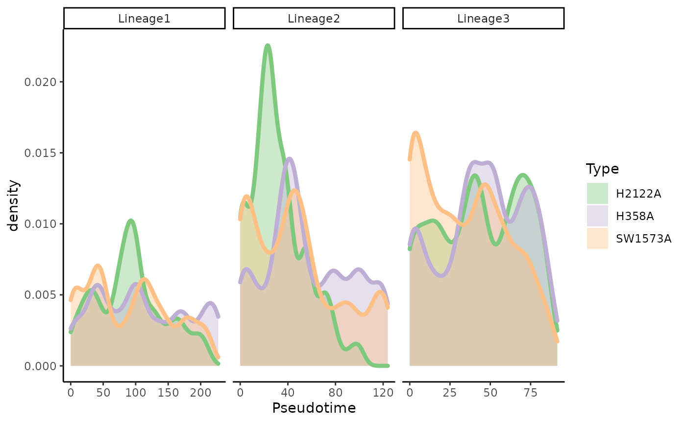
Visually, we can see three phenomenons:
- In lineage 1, there is a cluster of cells from H2122A around pseudotime 100, and more cells at the end of the lineage for condition H358A.
- In lineage 2, there are many more cells from H2122A for earlier pseudotime values and far fewer for later time points.
- In lineage 3, there are many more cells from SW1573A for earlier pseudotime values and far fewer for later time points.
Test
We can also test this in a more principled manner using the progressionTest. Since we have three conditions, we perform a classifier test (see (Lopez-Paz and Oquab 2016)). By setting lineages=TRUE, we perform the test for individual lineages and for the full trajectory.
The test statistic reflects the accuracy of the classifier on a balanced test data, so under the null, the expected value is \(1/3\).
progressionTest(sds, conditions = kras$Batch, lineages = TRUE)## lineage statistic p.value
## 1 All 0.8296334 0.000000e+00
## 2 1 0.5089786 2.355639e-43
## 3 2 0.4859742 2.520532e-15
## 4 3 0.4549123 1.840264e-11Differential Differentiation
Each cell in a trajectory is characterized with two components: its pseudotime values in each lineage, and its weights with regard to each lineage. Differential progression looks at the distribution of pseudotime between conditions while differential differentiation looks at the distribution of weights values between conditions.
It is slightly harder to interpret but we can start with a few plots.
Plot
df <- bioc2021trajectories::sling_reassign(sds) %>%
  as.data.frame() %>%
  mutate(cells = rownames(.)) %>%
  dplyr::rename("Lineage1" = V1, "Lineage2" = V2, "Lineage3" = V3) %>%
  pivot_longer(starts_with("Lineage"), names_to = "Curve", values_to = "weights") %>%
  full_join(df) %>%
  group_by(cells) %>%
  select(-pst) %>%
  mutate(weights = weights / sum(weights)) %>%
  ungroup()
## Setting options('download.file.method.GEOquery'='auto')## Setting options('GEOquery.inmemory.gpl'=FALSE)## Joining, by = c("cells", "Curve")We can first look at the total weight of each lineage in each condition. Two clear conclusions can be drawn here: + Lineage 1, the longest lineage, indeed captures more cells in all lineages + There are fewer H2122A cells in lineage 2, compared to the other conditions.
ggplot(df %>% group_by(Batch, Curve) %>%
         summarise(weights = mean(weights), .groups = NULL),
       aes(x = Curve, fill = Batch, y = weights)) +
  geom_col(position = "dodge") +
  scale_fill_brewer(palette = "Accent") +
  theme(legend.position = c(.7, .7)) +
  labs(x = "", y = "Mean weight")
## `summarise()` has grouped output by 'Batch'. You can override using the `.groups` argument.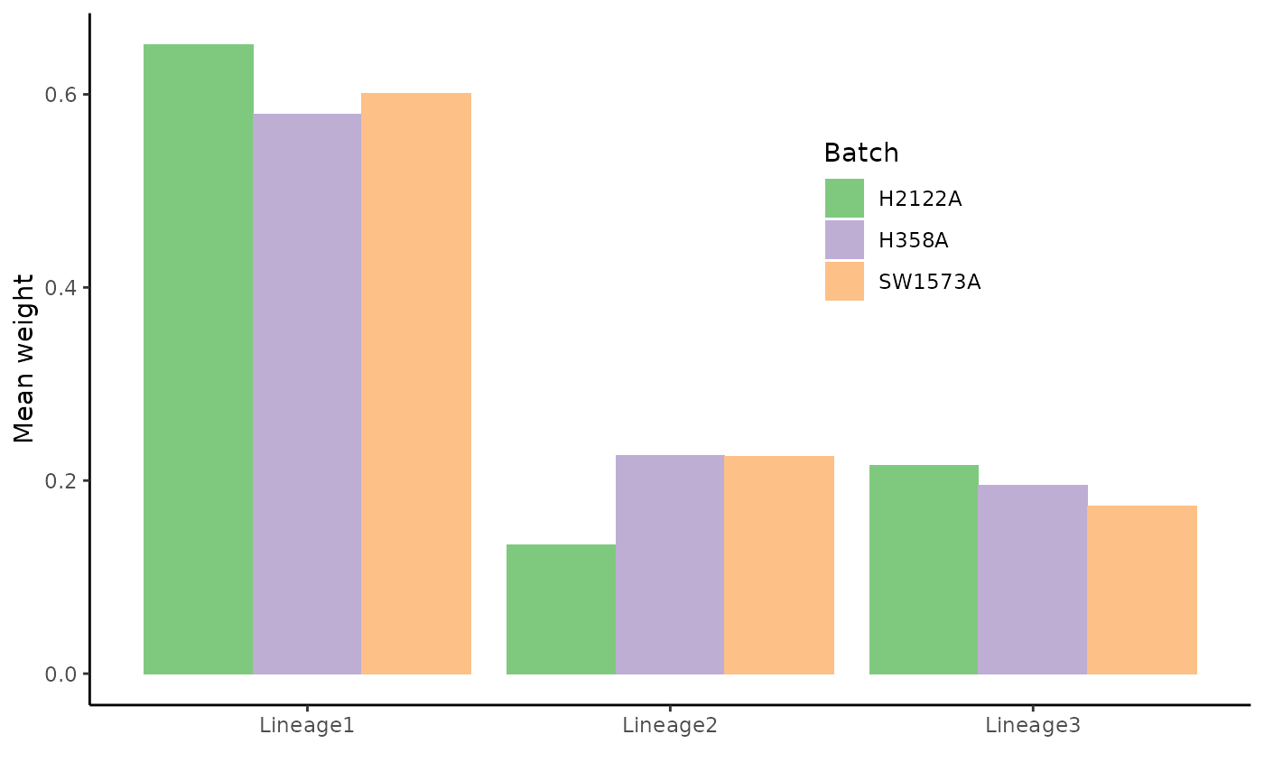
ggplot(df %>% pivot_wider(names_from = "Curve", values_from = "weights"),
       aes(x = Lineage1, y = Lineage3)) +
  geom_hex() +
  scale_fill_viridis_c(direction = -1) +
  facet_wrap(~Batch, scales = "free") +
  geom_abline(slope = -1, intercept = 1, linetype = "dotted") +
  geom_abline(slope = -1, intercept = 2/3, linetype = "dotted") +
  geom_abline(slope = -1, intercept = 1/3, linetype = "dotted") +
  annotate("text", x = .53, y = .53, label = "w3 = 0", angle = -52) +
  annotate("text", x = .62, y = .1, label = "w3 = 1/3", angle = -52) +
  annotate("text", x = .14, y = .14, label = "w3 = 2/3", angle = -52) +
  theme(legend.position = "bottom") +
  labs(x = "Weights for Lineage 1 (w1)", y = "Weights for Lineage 2 (w2)",
       fill = "counts per hexagon")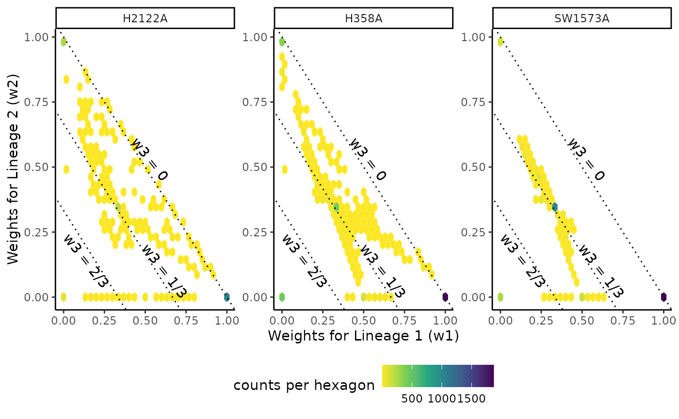
Test
differentiationTest(sds, conditions = kras$Batch, pairwise = TRUE)## note: only 1 unique complexity parameters in default grid. Truncating the grid to 1 .
##
## note: only 1 unique complexity parameters in default grid. Truncating the grid to 1 .
##
## note: only 1 unique complexity parameters in default grid. Truncating the grid to 1 .
##
## note: only 2 unique complexity parameters in default grid. Truncating the grid to 2 .## pair statistic p.value
## 1 All 0.4900000 8.231091e-42
## 2 1vs2 0.4210231 6.586841e-13
## 3 1vs3 0.4042857 5.557279e-10
## 4 2vs3 0.4793883 9.359587e-18Session info
## R version 4.1.0 (2021-05-18)
## Platform: x86_64-pc-linux-gnu (64-bit)
## Running under: Ubuntu 20.04.2 LTS
##
## Matrix products: default
## BLAS/LAPACK: /usr/lib/x86_64-linux-gnu/openblas-pthread/libopenblasp-r0.3.8.so
##
## locale:
##  [1] LC_CTYPE=en_US.UTF-8       LC_NUMERIC=C
##  [3] LC_TIME=en_US.UTF-8        LC_COLLATE=en_US.UTF-8
##  [5] LC_MONETARY=en_US.UTF-8    LC_MESSAGES=C
##  [7] LC_PAPER=en_US.UTF-8       LC_NAME=C
##  [9] LC_ADDRESS=C               LC_TELEPHONE=C
## [11] LC_MEASUREMENT=en_US.UTF-8 LC_IDENTIFICATION=C
##
## attached base packages:
## [1] stats4    stats     graphics  grDevices utils     datasets  methods
## [8] base
##
## other attached packages:
##  [1] caret_6.0-88                lattice_0.20-44
##  [3] ggplot2_3.3.5               tidyr_1.1.3
##  [5] cowplot_1.1.1               pheatmap_1.0.12
##  [7] RColorBrewer_1.1-2          condiments_1.1.02
##  [9] slingshot_2.1.0             TrajectoryUtils_1.1.0
## [11] princurve_2.1.6             SingleCellExperiment_1.15.1
## [13] SummarizedExperiment_1.23.1 Biobase_2.53.0
## [15] GenomicRanges_1.45.0        GenomeInfoDb_1.29.3
## [17] IRanges_2.27.0              S4Vectors_0.31.0
## [19] BiocGenerics_0.39.1         MatrixGenerics_1.5.1
## [21] matrixStats_0.59.0          tradeSeq_1.7.03
## [23] dplyr_1.0.7
##
## loaded via a namespace (and not attached):
##   [1] systemfonts_1.0.2           plyr_1.8.6
##   [3] igraph_1.2.6                splines_4.1.0
##   [5] BiocParallel_1.27.0         bioc2021trajectories_0.0.21
##   [7] digest_0.6.27               foreach_1.5.1
##   [9] htmltools_0.5.1.1           viridis_0.6.1
##  [11] fansi_0.5.0                 magrittr_2.0.1
##  [13] memoise_2.0.0               tensor_1.5
##  [15] openxlsx_4.2.4              limma_3.49.1
##  [17] readr_1.4.0                 recipes_0.1.16
##  [19] gower_0.2.2                 R.utils_2.10.1
##  [21] pkgdown_1.6.1               spatstat.sparse_2.0-0
##  [23] colorspace_2.0-2            textshaping_0.3.5
##  [25] xfun_0.24                   hexbin_1.28.2
##  [27] crayon_1.4.1                RCurl_1.98-1.3
##  [29] spatstat_2.2-0              spatstat.data_2.1-0
##  [31] GEOquery_2.61.0             survival_3.2-11
##  [33] iterators_1.0.13            glue_1.4.2
##  [35] polyclip_1.10-0             gtable_0.3.0
##  [37] ipred_0.9-11                zlibbioc_1.39.0
##  [39] XVector_0.33.0              DelayedArray_0.19.1
##  [41] Ecume_0.9.1                 kernlab_0.9-29
##  [43] Rhdf5lib_1.15.2             DropletUtils_1.13.1
##  [45] HDF5Array_1.21.0            abind_1.4-5
##  [47] scales_1.1.1                edgeR_3.35.0
##  [49] Rcpp_1.0.6                  viridisLite_0.4.0
##  [51] dqrng_0.3.0                 spatstat.core_2.2-0
##  [53] proxy_0.4-26                lava_1.6.9
##  [55] prodlim_2019.11.13          ellipsis_0.3.2
##  [57] scuttle_1.3.0               R.methodsS3_1.8.1
##  [59] pkgconfig_2.0.3             farver_2.1.0
##  [61] nnet_7.3-16                 deldir_0.2-10
##  [63] locfit_1.5-9.4              utf8_1.2.1
##  [65] tidyselect_1.1.1            labeling_0.4.2
##  [67] rlang_0.4.11                reshape2_1.4.4
##  [69] munsell_0.5.0               tools_4.1.0
##  [71] cachem_1.0.5                generics_0.1.0
##  [73] evaluate_0.14               stringr_1.4.0
##  [75] fastmap_1.1.0               yaml_2.2.1
##  [77] ragg_1.1.3                  goftest_1.2-2
##  [79] ModelMetrics_1.2.2.2        transport_0.12-2
##  [81] knitr_1.33                  fs_1.5.0
##  [83] zip_2.2.0                   randomForest_4.6-14
##  [85] purrr_0.3.4                 RANN_2.6.1
##  [87] pbapply_1.4-3               nlme_3.1-152
##  [89] sparseMatrixStats_1.5.0     R.oo_1.24.0
##  [91] xml2_1.3.2                  compiler_4.1.0
##  [93] e1071_1.7-7                 spatstat.utils_2.2-0
##  [95] spatstat.linnet_2.2-1       tibble_3.1.2
##  [97] stringi_1.6.2               highr_0.9
##  [99] desc_1.3.0                  Matrix_1.3-4
## [101] vctrs_0.3.8                 pillar_1.6.1
## [103] lifecycle_1.0.0             rhdf5filters_1.5.0
## [105] spatstat.geom_2.2-0         data.table_1.14.0
## [107] bitops_1.0-7                R6_2.5.0
## [109] gridExtra_2.3               codetools_0.2-18
## [111] MASS_7.3-54                 rhdf5_2.37.0
## [113] rprojroot_2.0.2             withr_2.4.2
## [115] GenomeInfoDbData_1.2.6      hms_1.1.0
## [117] mgcv_1.8-36                 parallel_4.1.0
## [119] beachmat_2.9.0              grid_4.1.0
## [121] rpart_4.1-15                timeDate_3043.102
## [123] class_7.3-19                rmarkdown_2.9
## [125] DelayedMatrixStats_1.15.0   pROC_1.17.0.1
## [127] lubridate_1.7.10